9. Visualización

1 Visualización: gramática de ggplot2 → ggplotly → plotly

Objetivo: entender la gramática de los gráficos en ggplot2, crear dos gráficos sencillos, dejar un apartado para enlazar o embeber tu clase completa en HTML, y mostrar cómo convertir y crear gráficos interactivos con ggplotly y la gramática nativa de plotly en R.

---

1.1 La gramática de ggplot2 (mapa mental)

Tip

Gramática base:
ggplot(data, aes(mapeos)) + geom_*() + stat_*() + scale_*() + coord_*() + facet_*() + theme_*() + labs()

• data: el data.frame que contiene tus variables.
  
• aes(): mapeos estéticos (ej. x, y, color, fill, size, shape).
  
• **geom_*():** geometrías (puntos, barras, líneas, boxplots…).
  
• **stat_*():** transformaciones estadísticas (bins, densidad, smooth…), muchas ya vienen “dentro” del geom.
  
• **scale_*():** controles de escalas, etiquetas y paletas (eje log, comas, porcentajes).
  
• **coord_*():** sistemas de coordenadas (flip, polar, limits).
  
• **facet_*():** paneles por subgrupos (facet_wrap, facet_grid).
  
• **theme_*() / theme():** estilos visuales y ajustes finos.
  
• labs(): títulos, subtítulos, ejes, leyendas.

Code

library(tidyverse)

Warning: package 'tidyverse' was built under R version 4.2.2

Warning: package 'ggplot2' was built under R version 4.2.3

Warning: package 'tibble' was built under R version 4.2.3

Warning: package 'tidyr' was built under R version 4.2.2

Warning: package 'purrr' was built under R version 4.2.2

Warning: package 'stringr' was built under R version 4.2.3

Warning: package 'forcats' was built under R version 4.2.2

Warning: package 'lubridate' was built under R version 4.2.2

── Attaching core tidyverse packages ──────────────────────── tidyverse 2.0.0 ──
✔ forcats   1.0.0     ✔ stringr   1.5.1
✔ ggplot2   3.5.1     ✔ tibble    3.2.1
✔ lubridate 1.9.2     ✔ tidyr     1.3.0
✔ purrr     1.0.1     
── Conflicts ────────────────────────────────────────── tidyverse_conflicts() ──
✖ dplyr::filter() masks stats::filter()
✖ dplyr::lag()    masks stats::lag()
ℹ Use the conflicted package (<http://conflicted.r-lib.org/>) to force all conflicts to become errors

Code

library(ggplot2)

# Base mínima por si no existe:
if (!exists("BaseSal")) {
  suppressWarnings({
    if (!exists("Salaries")) {
      library(readxl)
      if (file.exists(ruta_salaries)) {
        Salaries <- readxl::read_excel(ruta_salaries)  
      } else {
        # muestra didáctica si no hay archivo
        Salaries <- tibble(
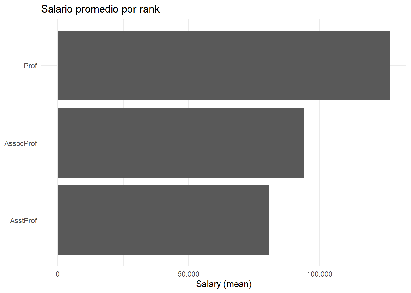
          rank = sample(c("AsstProf","AssocProf","Prof"), 120, TRUE),
          sex  = sample(c("Female","Male"), 120, TRUE),
          `yrs.service` = sample(1:30, 120, TRUE),
          salary = round(rlnorm(120, 11, 0.25), 0)
        )
      }
    }
    BaseSal <- dplyr::select(Salaries, dplyr::any_of(c("rank","sex","yrs.service","salary")))
  })
}

1.2 Dos gráficos sencillos con ggplot2

• 1. Dispersión con iris

Code

p_iris <- ggplot(iris, aes(x = Sepal.Length, y = Sepal.Width, color = Species)) +
  geom_point() +
  theme_minimal() +
  labs(title = "Iris: Sepal Length vs Width", x = "Sepal.Length", y = "Sepal.Width", color = "Species")
p_iris

• 2. Barras: salario promedio por rank

Code

library(scales)  # para etiquetas con comas

Warning: package 'scales' was built under R version 4.2.3

Attaching package: 'scales'

The following object is masked from 'package:purrr':

    discard

The following object is masked from 'package:readr':

    col_factor

Code

prom_rank <- BaseSal %>%
  group_by(rank) %>%
  summarise(mean_salary = mean(salary, na.rm = TRUE), .groups = "drop")

p_sal <- ggplot(prom_rank, aes(x = reorder(rank, mean_salary), y = mean_salary)) +
  geom_col() +
  coord_flip() +
  scale_y_continuous(labels = label_comma()) +
  theme_minimal() +
  labs(title = "Salario promedio por rank", x = NULL, y = "Salary (mean)")
p_sal

Note

Clase completa: consulta/estudia la clase extendida aquí:
➡️ Ir a la clase completa (HTML)

1.3 Interactividad rápida con ggplotly (sobre un ggplot)

Code

library(plotly)

Warning: package 'plotly' was built under R version 4.2.3

Attaching package: 'plotly'

The following object is masked from 'package:ggplot2':

    last_plot

The following object is masked from 'package:stats':

    filter

The following object is masked from 'package:graphics':

    layout

Code

# Convertir el scatter de ggplot en interactivo:
p_iris_inter <- ggplotly(p_iris)
p_iris_inter

Code

# También puedes convertir el barplot:
ggplotly(p_sal)

1.4 Gramática nativa de plotly en R (sin ggplot)

Tip

Esquema de plotly (R): plot_ly(data, x = ~varx, y = ~vary, type = “scatter”/“bar”/…, mode = “markers”/“lines”) %>% add_*() %>% layout(…)

~ indica mapeo de columnas del data.frame.

add_markers(), add_lines(), add_bars(), etc., añaden trazas.

layout() ajusta títulos, ejes, leyendas y márgenes.

Code

# Dispersión interactiva con mtcars (nativo plotly)
p_plotly <- plot_ly(
  data = mtcars,
  x = ~wt, y = ~mpg,
  type = "scatter", mode = "markers",
  color = ~factor(gear),  # mapea color a 'gear' como factor
  text = ~paste("Modelo:", rownames(mtcars))  # tooltip
) %>%
  layout(
    title = "mtcars: Consumo vs Peso (plotly nativo)",
    xaxis = list(title = "Peso (1000 lb)"),
    yaxis = list(title = "Millas/galón"),
    legend = list(title = list(text = "Gears"))
  )

p_plotly

Tip

usa ggplot2 cuando quieras una gramática declarativa y un tema consistente; usa ggplotly para interactividad rápida sobre gráficos ya definidos; o plotly nativo si quieres controlar a detalle interacciones y capas desde el inicio (trazas).